General information regarding the predictive calculation of the sound absorption coefficient and sound reduction index of multilayer acoustic walls using SILDIS® software
The SILDIS®[0] software (in Excel format) enables the predictive computation of the sound absorption coefficient and of the sound reduction index of multilayer acoustic walls combining porous media, cloths (surfacings), perforated protections (protective layers) and - in the sole case of the evaluation of the sound transmission loss - possibly with the consideration of thin plates for the modeling of acoustical behaviour of various construction and soundproofing products & systems:
- partition walls
- panels
- linings
- laggings with additionnal skin
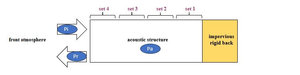
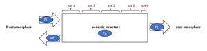
Such a calculation requires taking into account, upstream of the acoustic structure, a fluid (front atmosphere), and downstream, possibly: an impervious rigid back or a fluid (rear atmosphere). For each of these configurations, Figures 1 and 2 below illustrate (respectively) the paths of the acoustic waves and the associated sound pressures:
- Pi: sound pressure of the incident wave
- Pr: sound pressure of the reflected wave
- Pi: sound pressure of the absorbed wave
- Pt: sound pressure of the transmitted wave (only in the case of a downstream atmosphere)
|
Figure 1 Acoustic waves and associated acoustic pressures in the presence of an impervious rigid back behind an acoustic structure, for the calculation of the sound absorption coefficient using SILDIS® software |
|
Figure 2 Acoustic waves and associated sound pressures in the presence of a fluid (rear atmosphere) behind an acoustic structure, for the calculation of the sound absorption coefficient and of the sound reduction index using SILDIS® software |
In relation to these sound wave paths and the associated acoustic pressures, various frequency-dependent quantities must be considered (and not only for plane waves):
- the acoustic reflection factor (in terms of pressure) R = Pr/Pi (a dimensionless complex quantity); the acoustic absorption coefficient α = 1 - |R|² (a dimensionless real number)
- the sound transmission factor τ = |Pt/Pi|² (a dimensionless real number); the sound reduction index R = -10 log(τ) (a real number expressed in dB)
Another page on this site[1] provides detailed information regarding:
- the characteristics considered for each material layer (nature, model(s), thickness, temperature)
- the properties of the upstream atmosphere and the downstream environment (depending on the simulation context: axis of symmetry, impervious rigid back, or rear atmosphere)
- the software's modeling capabilities
- the naming conventions for Excel sheets used for data input, output visualization (e.g. calculation results), or both tasks combined
- the "internal use" and "external use" operating modes
Thus, for both "internal use" and "external use," the input data to be entered are:
- in the "in-COALA" Excel sheet (and, where applicable - for certain special plates - into other related sheets): characteristics and properties listed above
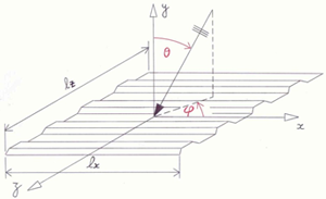
For envisaged calculations, the geometry used is shown in Figure 3 (illustrating the case of a profiled facing):
- axes
- x: for an orthotropic plate, the direction of highest flexural rigidity (xx: axis about which the flexural rigidity of the orthotropic plate is minimal)
- y: direction of the wall thickness (yy: axis perpendicular to the wall surface)
- z: for an orthotropic plate, the direction of lowest flexural rigidity (zz: axis about which the flexural rigidity of the orthotropic plate is maximal)
- angles
- orientation relevant to an orthotropic plate: the angle φ (may be displayed as: fi) of the projection (onto the surface of the acoustic structure) of the wave propagation direction in the front atmosphere, measured relative to the xx axis (e.g. for a corrugated acoustic structure, this is the angle relative to the axis parallel to the corrugations, as shown in the figure)
- incidence: the angle θ (may be displayed as: teta) of the wave propagation direction in the front atmosphere, measured relative to the yy axis
|
Figure 3 Geometry considered for the calculation of the sound absorption coefficient and of the sound reduction index/transmission loss of multilayer walls using SILDIS® software |
For "internal use" as for "external use", the predictive computation of the sound absorption coefficient (in normal or statistical incidence and in the sense of W.C. Sabine) and of the sound reduction index (sound transmission loss) involves different Excel sheets, depending on current needs for displaying performance indicators.
Summary of Excel sheets in relation to the predictive computation of the sound absorption coefficient and of the sound reduction index with the SILDIS® software for "internal use" and for "external use"
| Excel sheet | Index of considered sets | Materials considerated (possibly) | At the rear of the acoustic structure | Performance indicator displayed |
| in-out COPPA0 | 1 to imax | porous media, cloths (surfacings), perforated protections (protective layers) (0 thin plate);infinite partition wall area |
impervious rigid back |
For plane absorber - Sound absorption coefficient (for normal incidence), and also surface impedance |
| in-out COPPA0+ | 1 | porous media, cloths (surfacings), perforated protections (protective layers) (0 thin plate);infinite partition wall area |
impervious rigid back |
For plane or curved absorber - Sound absorption coefficient (for normal incidence), and also surface impedance |
| in-out COPPA1 | 0 | all in all: 1 thin plate; infinite or finite partition wall area (consideration of dimensions separeaely) |
rear atmosphere |
For plane absorber - Sound reduction index/transmission loss (for diffuse field) |
| in-out COPPA2 | 0 and 2 |
2 thin plates and two intermediate porous media; infinite wall area regarding the plates and the porous media
|
rear atmosphere |
For plane absorber - Sound reduction index/transmission loss (for diffuse field) |
| in-out COPPA | 0 to imax | pporous media, cloths (i.e. facings), perforated protections (i.e. perforated protective layers), thin plates: infinite wall area if the 90° model is chosen for the integration limit θL; otherwise finite wall with consideration of the product of dimensions (if the DAV model is chosen). |
symmetry axis/impervious rigid back or rear atmosphere |
For flat absorbers - Sound absorption coefficient (for normal or statistic/random incidence, in the sense of W.C. Sabine), weighted sound absorption coefficient (single-number rating) αw, absorption class, and also NRC, SAA For flat absorbers - Sound reduction index (for statistic/random incidence), weighted sound reduction index (including spectrum adaptation terms), and also insertion loss relative to a set 0 plate and sound power radiated by the panel |
With reference to the information in the table above, it is possible to consider the following regarding laboratory-measurable acoustic performance indicators:
- the "in-out COPPA0" Excel sheet displays results from a Kundt's tube measurement simulator; the "in-out COPPA0+" Excel sheet extends this concept to curved absorbers (subject to the actual availability of the equipment in question)
- the "in-out COPPA" Excel sheet displays results from a simulator for measurement in a Kundt' tube, a reverberation room, and a test rig designed to characterize acoustic transmission loss; the "in-out COPPA1" and "in-out COPPA2" Excel sheets display results from a measurement simulator for a test rig designed to characterize acoustic transmission loss, specifically for single-leaf and double-leaf partitions, respectively
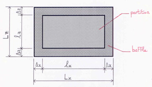
For walls of finite dimensions, the geometry under consideration is illustrated in Figure 4 (in relation to the configuration of some test benches found here and there).
|
Figure 4 geometry of a wall for mounting with a frame (baffle) |
In general:
- for Lx ≠ lx, the following limitation on input data is required: Int [π 0.5 * Lx * 20,000 / c0] ≤ 464
- for Lz ≠ lz, the following limitation on input data is required: Int [π 0.5 * Lz * 20,000 / c0] ≤ 464
In the above, c0 is the speed of sound in air (m/s).
In particular:
- for Lx ≠ lx (or Lz ≠ lz), the following input data constraint applies to Lx (or Lz): 4.500 m when c0 = 343.3 m/s
Regarding the angle of incidence, the calculation involves integrating over the limit values of the relevant angles:
- regarding orientation (angle φ): integration is performed from φmin to φmax, values selected by the user (to match actual conditions) from a predefined list (in the current program version: angles from 5.625° to 84.375° with an increment of 11.25°, i.e. N=8 angles)
- reminder: orientation (angle φ) is relevant for orthotropic plates integrated into the acoustic structure
- regarding incidence (angle θ): integration is performed from θmin to min(θmax, θL)
- θmin and θmax are selected by the user (to match actual conditions) from a predefined list (in the current program version: angles from 0° to 89.375° with an increment of 1.25°, i.e. 73 angles)
- θL is determined based on various models, as shown in the table below
Summary of limit angle (θL) sub-models in the "in-out COPPA" Excel sheet of the SILDIS® software
| Sub-model | 90° | DAV | MOI |
| Comment(s) | θL = 90° |
θL variable depending on frequency and wall area
|
θL variable depending on frequency and wall area |
Consequently:
- regarding orientation (angle φ):
- for a simulation between two limiting angles of incidence (user-defined), the user can enter (via a drop-down menu) a value for φmin and a value for φmax
- for a simulation for diffuse incidence (with respect to the orientation angle φ), the user can enter (via a drop-down menu) 5.625° for φmin and 84.375° for φmax
- regarding incidence (angle θ):
- for a simulation between two limiting angles of incidence (user-defined), without further considerations, the user can enter(via a drop-down menu):
- for θmin and a value for θmax: a user-defined value
- for θL: the 90° sub-model o for a simulation involving an acoustic field such as that encountered in situ (diffuse?) (with respect to the angle of incidence θ)
- using the (classical) approach that employs - for a wall of undefinite dimensions - a single limiting angle of incidence (78°, 80°, 85°... in all cases less than 90° to reduce discrepancies between predicted and measured results, particularly at low frequencies), the user can enter (via a drop-down menu):
- for θmin: 0°
- for θmax: the value closest (to the desired limiting angle)
- for θL: the 90° sub-model
- using the "original" approach underlying the DAV model (which accounts for partition dimensions), the user can enter(via a drop-down menu):
- for θmin: 0°
- for θmax: 90°
- for θL: the DAV sub-model
- if he prefers not to replace the denominator of the integration formula used (see below) with 0.5, but is rather interested in the approach based on the modified DAV model, the user can enter (using a drop-down menu):
- for θmin: 0°
- for θmax: 90°
- for θL: the MOI sub-model (in September 2026: sub-model on hold)
- for a simulation between two limiting angles of incidence (user-defined), without further considerations, the user can enter(via a drop-down menu):
Thus, for both "internal use" and "external use," the input data required - relating to the geometry of the multilayer acoustic structure - for the predictive computation of the sound absorption coefficient and of the sound reduction index of walls are as follows:
- in the "in-out COPPA0" Excel sheet: none
- in the "in-out COPPA0+" Excel sheet: none
- in the "in-out COPPA1" Excel sheet: none
- in-out COPPA2" Excel sheet: none
- in the "in-out COPPA" Excel sheet (used without new entry in "in-out COPPA1" and in the "in-out COPPA2" Excel sheets):
- dimensions of the frame (baffle) in which the partition is symmetrically mounted: Lx in the x-direction (m) and Ly in the z-direction (m)
- dimensions of the partition: lx in the x-direction (m) and ly in the z-direction (m)
- orientation (angle φ): angular integration limits φmin and φmax (for an "external use": respectively 5.625° and 84.375°; this choice is inconsequential in case of an isotropic partition wall, being relevant only in case of orthotropic partions walls)
- incidence (angle θ): angular integration limits θmin and θmax and sub-model for θL
Calculations are performed within the 20 Hz - 20 kHz frequency range using 1/21-octave frequency bands, which form the basis for the displayed curves. Values for one-third-octave bands (center frequencies from 20 Hz to 20 kHz) and octave bands (center frequencies from 31.5 Hz to 16 kHz) are presented in tabular form.
Predictive computation of the sound absorption coefficient for multilayer acoustic walls using SILDIS® software
Using the SILDIS® software, sound absorption can be characterized by three main performance indicators (taking frequency into account):
- normal-incidence sound absorption coefficient (α₀)
- statistical-incidence i.e. random incidence sound absorption coefficient (αstat)
- Sabine absorption coefficient/factor (αsab)
Predictive computation of the sound absorption coefficient for normal incidence (αo) of multilayer acoustic walls using SILDIS® software
The normal-incidence sound absorption coefficient (α₀) - as displayed in the "in-out COPPA0", "in-out COPPA0+", and "in-out COPPA" Excel sheets when selecting θmin = θmax = 0° - is defined as the ratio of the sound power absorbed by the surface of the considered partition (i.e. the power not reflected) to the incident sound power. The computation is:
- based on the surface impedance of the multilayer acoustic structure calculated for the outermost layer of the set with index i ≤ imax (where imax is the maximum set index selected by the user)
- performed assuming θ = 0°
In the case of an impervious rigid back, the calculated values for various indicators are - provided appropriate input settings are selected in the software regarding angular integration limits - comparable to those obtained from standardized measurements (with a Kundt's tube):
- cf. ISO 10534-1: Acoustics - Determination of sound absorption coefficient and impedance in impedance tubes – Part 1: Method using standing wave ratio
Predictive computation of the sound absorption coefficient for statistic/random incidence (αo) of multilayer acoustic walls using SILDIS® software
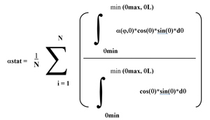
The sound absorption coefficient for statistic/random incidence (αstat) - as displayed in the "in-out COPPA" Excel sheet - is defined as the ratio of the sound power absorbed by the surface of the wall in question (i.e. not reflected) to the incident sound power, considering all possible angles of incidence with equal probability within specific angular limits. The calculation is:
- based on the surface impedance of the multilayer acoustic structure, calculated for the outermost layer of the set with index i ≤ imax (where imax is the maximum set index selected by the user)
- performed via angular integration (with respect to angles φ and θ, for averaging) using the generalized Formula 1 below, with the notable exception of the case where the DAV sub-model is used for θL (in which case the denominator is replaced by 0.5)
In the case of an impervious rigid back, the calculated results for various indicators are - provided appropriate input settings are selected in the software regarding angular integration limits - comparable to those obtained from standardized measurements:
- cf. ISO 354 Acoustics – Measurement of sound absorption in a reverberation room
|
Formula 1 |
Predictive computation of the Sabine factor/coefficient (αsab) of multilayer acoustic walls using SILDIS® software
The Sabine factor/coefficient (αsab) - as displayed in the "in-out COPPA" Excel sheet -is defined as the ratio of the equivalent sound absorption area of a sample to the area of the sample.
The calculation is performed by extrapolating the αstat coefficient, using a user-selected αsabmax value.
In the case of an impervious rigid back, the calculated results for various indicators are - provided appropriate input settings are selected in the software regarding angular integration limits - comparable to those obtained from standardized measurements:
Sabine factor/coefficient (αsab) - as displayed in the "in-out COPPA" Excel sheet -: ISO 354 Acoustics – Measurement of sound absorption in a reverberation room
- weighted sound absorption coefficient αw and absorption class - as displayed in the "in-out COPPA" Excel sheet -: cf. ISO 11654 Acoustics – Sound absorbers for use in buildings – Rating of sound absorption
Input data for the predictive computation of the sound absorption coefficient of multilayer walls using SILDIS® software
For both "internal use" and "external use," the input data to be entered - in addition to the data regarding the geometry of the multilayer acoustic structure (the latter being listed above) - are as follows regarding the sound absorption of a wall:
- in the "in-out COPPA0" Excel sheet: none
- in the "in-out COPPA0+" Excel sheet: none
- in the "in-out COPPA1" Excel sheet: not applicable
- in the "in-out COPPA2" Excel sheet: not applicable
- in the "in-out COPPA" Excel sheet: the maximum value for αsab
Predictive computation of the sound reduction index for multilayer acoustic walls using SILDIS® software
Using the SILDIS® software, sound reduction index can be characterized by three main performance indicators (taking frequency into account):
- the diffuse-field sound reduction index (Rdif) for a monolithic element (a single thin panel)
- the diffuse-field sound reduction index (Rdif) for two sets of adjacent thin plates (unbonded) with two intermediate porous layers
- the statistical-incidence sound reduction index (Rstat)
The A-weighted overall values expressed in dB(A) are calculated relative to the reference spectrum (Lw0, selected by the user and entered in 1/3-octave or octave bands in the "in COALA" Excel sheet).
Various parameters can be taken into account using different models and settings - entered once and reused -including, where applicable, for the calculation of the three performance indicators related to the sound reduction of partitions (common sub-models and settings linked to sound reduction).
Summary of COMMON sub-models and settings linked to sound reduction in the "in-out COPPA" Excel sheet of the SILDIS® software for "internal use" and "external use."
| Parameter | eigenfrenquency of the first plate bending mode f11 | Leaks: slit models (m) |
| Sub-models | HAN HEA |
GOM (transmission factor variable depending on frequency) UNI (transmission factor set to 1 for all frequencies) |
For an "internal use" as for "external use" the input data required - in addition to those relating to the geometry of the multilayer acoustic structure (the latter being listed above) - regarding the sound reduction of a wall are in the "in-out COPPA" Excel sheet (used without new entry in "in-out COPPA1" and in the "in-out COPPA2" Excel sheets):
- a model for calculating the eigenfrenquency of the first plate bending mode f11
- if and only if slits are taken into account:
- slit length (m)
- slit width (m)
Predictive computation of sound reduction index for diffuse acoustic field (Rdif) for a monolithic element (1 single thin plate) using SILDIS® software
The diffuse-field sound reduction index (Rdif) for a monolithic element (a single thin platel) - as displayed in the "in-out COPPA1" Excel sheet - is defined as ten times the base-10 logarithm of the ratio of the sound power incident on a partition to the sound power transmitted by the sample (1/τdif).
Except when sub-model INT is used, the calculation is performed without angular integration within the SILDIS® calculation routines, relying instead on results from published literature.
Various parameters can be accounted for using different sub-models and settings e.g. depending on the critical frequency fc (Hz) where or the speed of the free bending waves in the plate equals the speed of sound in the surrounding porous medium (fluid), involving a remarkable dip in the sound reduction index curve plotted against frequency (for an incidence angle differing from 0°).
Summary of sub-models and settings in the "in-out COPPA1" Excel sheet of the SILDIS® software for "internal use" and "external use"
| Parameter | Boundary conditions | Radiation factor for free bending waves | Simplified transmission factor for normal incidence (0/1) | General model (for Rdif) | For f<fc, model for forced transmission | Model for resonant transmission | For f≈fc, model for transmission | Frequency range where f≈fc (in number of 1/3 oct frequency bands below fc) | For f>fc model for transmission | For f≈fc, model for transmission | Fequency range where f≈fc (in number of 1/3 oct frequency bands below fc) |
| Sub-models and settings | SSE i.e. Simply Supported Edges CE i.e. Clamped Edges MID i.e. MIDway from SSE and CE |
MAI NF |
0 1 |
SHA MOI |
4τ0 3τ0 INT SEW BAL DAV JOS GER NF NF2 NI1 NI2 ZER i.e. 0 |
SEA JOS NF NF2 NI1 NI2 ZER i.e. 0 |
JOS NF NAT |
0 1/2 1 1 1/2 2 2 1/2 3 |
INT SEA CRE JOS NF NIL |
JOS NF NI2 NAT |
0 1/2 1 1 1/2 2 2 1/2 3 |
For "external use," the input data to be entered - in addition to those relating to the geometry of the multilayer acoustic structure and in addition to common sub-models and settings linked to sound reduction(the latter being listed above) - regarding the sound reduction of a monolithic wall (in the "in-out COPPA1" Excel sheet) are:
- (as of September 2026, a time when calculation routine modifications are underway) the general SHA model, for which the settings and sub-models in the table above are unnecessary
Predictive computation of sound reduction index for diffuse acoustic field (Rdif) for 2 thin plates with 2 intermediate porous layers (double leaf-partition) using SILDIS® software
The diffuse-field sound reduction index (Rdif) for 2 plates with two intermediate porous layers (double leaf-partition) - as shown in the "in-out COPPA2" Excel sheet - is defined as ten times the base-10 logarithm of the ratio of the incident sound power on the partition to the sound power transmitted by the sample (1/τdif).
The calculation is performed without angular integration within the SILDIS® calculation routines, relying instead on results from published literature.
Various parameters can be accounted for using different sub-models.
Summary of sub-models and settings in the "in-out COPPA2" Excel sheet of the SILDIS® software for "internal use" and "external use."
| Parameter | General model | Sub-model (for model DAV) | Model for linkage (for general models SHA1,SHA2,SHA3) | Modèle for compliance (for general model DAV) |
| Sub-models | FAH DAV SHA1 SHA2 SHA3 |
1990 2009 2012 |
L-L i.e. Line-Line L-P i.e. Line-Point P-P i.e. Point-Point |
BYO PWR ZER |
For an "external use", the recommended model(s) are those both underlined and shown in bold in the table above.
In addition, various inputs are required:
- for line connections
- distance between line connections (m)
- vibration transmission factor (not for general models FAH, DAV, SHA1, SHA2, SHA3)
- connection compliance for the DAV general model and the BYO compliance model (in m/N)
- for point connections (for models DAV, SHA1, SHA2, SHA3)
- number of connections per m² (m⁻²)
- vibration transmission factor (not for general models FAH, DAV, SHA1, SHA2, SHA3)
- connection compliance for the DAV general model and the BYO compliance model (in m/N)
For "external use," the input data required - in addition to the geometric parameters of the multilayer acoustic structure and in addition to common sub-models and settings linked to sound reduction(listed above) - regarding sound reduction for two unbonded adjacent panel assemblies and two intermediate porous media (in the "in-out COPPA2" Excel sheet) are:
- a general model for Rdif and, if and only if the chosen general model is DAV, a general sub-model
- a connection model
- for line connections: the distance between line connections (m)
- for point connections: the number of connections per m² (m⁻²)
- the vibration transmission factor (not applicable to the FAH, DAV, SHA1, SHA2, or SHA3 general models)
- connection compliance for the DAV general model, specifically the BYO compliance model (in m/N)
In the case of a rear atmosphere, the calculated results for various indicators are comparable to those obtained from standardized measurements (provided appropriate inputs regarding angular integration limits are selected in the software):
- sound reduction index Rstat/Rdif - as displayed in the "in-out COPPA1", "in-out COPPA2", and "in-out COPPA" Excel sheets-: cf. ISO 140-3 Acoustics - Measurement of sound insulation in buildings and of building elements — Part 3: Laboratory measurement of airborne sound insulation of building elements
- weighted sound reduction index Rw and adaptation terms C and Ctr - as displayed in the "in-out COPPA1", "in-out COPPA2", and "in-out COPPA" Excel sheets -: cf. ISO 717-1 Acoustics - Rating of sound insulation in buildings and of building elements - Part 1: Airborne sound insulation
Predictive computation of sound reduction index for statistic/random incidence (Rstat) for multilayer acoustic walls using SILDIS® software
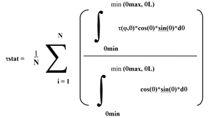
The incidence sound reduction index for statistical incidence i.e. for random incidence (Rstat) - as displayed in the "in-out COPPA" Excel sheet - is defined as ten times the decimal logarithm of the ratio between the acoustic power incident on the considered wall and the acoustic power transmitted by the sample 1/τstat.
The computation is:
- based on the surface impedance of the multilayer acoustic structure calculated for the upstream layer of the set with index i ≤ imax (where imax is the maximum set index selected by the user)
- performed by angular integration (with respect to angles φ and θ, for averaging) according to the generalized formula 2 below, with the notable exception of the case where the DAV submodel is used for θL (in which case the denominator is replaced by 0.5)
|
Formule 2 |
For "external use," the input data to be entered - in addition to those relating to the geometry of the multilayer acoustic structure and in addition to common sub-models and settings linked to sound reduction(the latter being listed above) - regarding the sound reduction index for statistic/randome incidence are:
- néant
In the case of a rear atmosphere, the calculated results for various indicators are (given an appropriate selection in the software of inputs for angular integration limits) comparable to those from standardized measurements:
- sound reduction index Rstat/Rdif - as displayed in the "in-out COPPA1," "in-out COPPA2," and "in-out COPPA" Excel sheets -: cf. ISO 140-3 Acoustics — Measurement of sound insulation in buildings and of building elements — Part 3: Laboratory measurement of airborne sound insulation of building elements
- weighted sound reduction index Rw and adaptation terms C and Ctr - as displayed in the "in-out COPPA1," "in-out COPPA2," and "in-out COPPA" Excel sheets -: cf. ISO 717-1 Acoustics — Rating of sound insulation in buildings and of building elements — Part 1: Airborne sound insulation
[0] Sound Impact Limitation - Design for Industrialized Solutions
[1] cf. Modeling and optimization of multilayer acoustic structures using SILDIS® software
 |
Désolé, le document téléchargeable ci-dessous n'a pas encore été traduit dans votre langage.
|
|